Excel 2016 Basics Chapter 5

In this tutorials we will cover Basics of excel 2016 like Cell references, Merging cells, Merging text with numbers, and Text to Columns Wizard. 

Relative, absolute and mixed cell references in Excel 2016 Basics

Many formulas in Excel contain references to other cells. These references allow formulas to dynamically update their contents.

We can distinguish three types of cell references: relative, absolute and mixed.

Relative cell references

This is the standard type of reference. Look at the following examples:

Example 1:

If cell A1 contains value 2, and cell B1 contains formula =A1+2 (referring to cell A1), then the formula B1 contains value 4. If you change the value in cell A1 to 5, then the value in cell B1 automatically changes to 7.

Example 2:

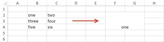
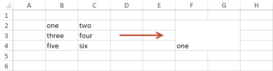
If cell B1 refers to cell A1, then after copying cell B1 to cell D2, the cell starts to refer to cell C2. In other words, cell reference has been moved by the same distance as the copied cell.

Example 3:

Look at the following example. Here, you can find the names of employees of a fictional company.

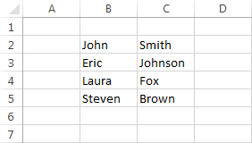
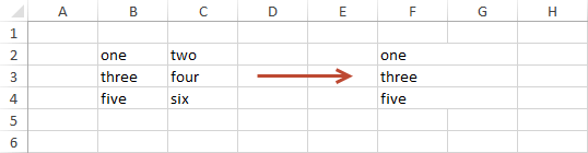
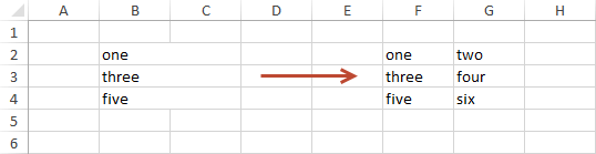
If you want to merge the first name with the last name and place them in column D, you don’t have to enter them manually, but you can merge them by using the relative references, instead.

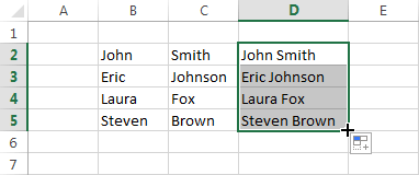
In this case, enter the formula =B2&” “&C2 into cell D2. It will merge cell B2, space, and cell C2. Now you can use AutoFill to fill the remaining cells.

You can display formulas instead of values by using the Ctrl + ` (the key that is located below the ESC key) keyboard shortcut.

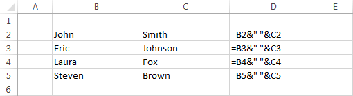
As you can see, only the formula in cell D2 refers to cells B2 and C2. References in the next cells have been shifted accordingly.

Absolute cell references

Absolute cell reference always points to the same place, even if you change the position of any of those cells. In other words, if you have cell A1 which refers to the contents of cell B1 (=$B$1) and then you change the position of A1 it will still refer to cell B1. If you drag cell B1 to another location, for example, B3, then A1 will point to the new location of the same cell (=$B$3).

Example 4:

Look at the following example: it shows the earnings of Tom Smith. We need to calculate how much tax he needs to pay each month.

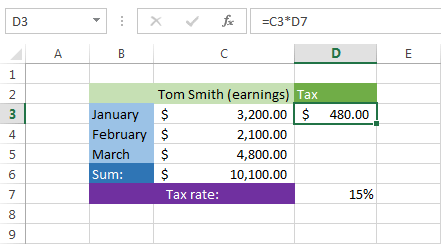
Look at the formula bar. It shows how much tax John needs to pay for January (=C3*D7). If you want to automatically fill the remaining months, you will notice that for February the reference doesn’t point to cell D7, instead, it points to cell D8, and for March to cell D9.

To create an absolute reference, click cell D3, then in the formula click text D7. Now press the F4 key and confirm it by pressing Enter. This will change a relative reference to an absolute reference.

Use AutoFill to count the taxes for February, March, then sum all the months. Press Ctrl + ` to display the formula.

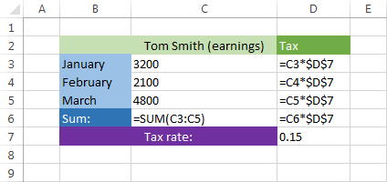
As you can see in the example above in all four cells, the first part of the formula is a relative cell reference and the second part is an absolute cell reference.

Mixed cell references

A mixed reference is a reference that refers to a specific row or column. For example, $A1 or A$1. If you want to create a mixed reference- press the F4 key on the formula bar two or three times depending on whether you want to refer to row or column. Press F4 one more time to go back to the relative cell reference.

Merging cells in Excel 2016 Basics

Merging cells in Excel can be useful when you want to format the look of your worksheet. You can merge two or more contiguous cells, both vertically and horizontally.

In order to do so, go to HOME >> Alignment >> Merge & Center. It’s a drop-down menu under which you will find four buttons:

Merge & Center

Merges selected cells into one larger cell while centering the text horizontally.

Merge Across

Select 6 cells (2×3) and merge them across. You will get 3 cells, one for each row.

Merge Cells

Merges cells into one larger, without centering its contents.

Unmerge Cells

If you want to unmerge previously merged cells, you can use this button.

Example:

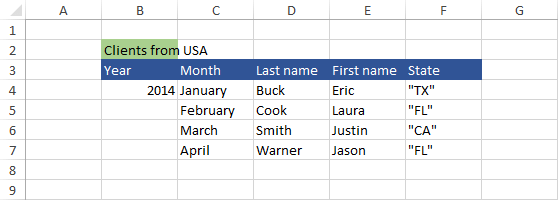
Look at the following example. It shows a list of customers from the USA. This table is not formatted in a proper way, so it doesn’t look very professional.

In order to format this table, do the following:

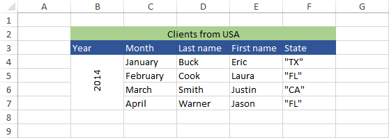
• Select cells from B2 to F2, then select the Merge & Center button,
• Now, select cells from B4 to B7, and once again select the Merge & Center,
• Go to HOME >> Alignment, click Middle Align, then choose HOME >> Alignment >> Rotate Text Up.

If you did everything correctly, you should get the following result.

NOTICE

• You can split only those cells that have been previously merged.
• When you merge multiple cells into one, only the value of the cell in the upper-left corner is preserved.
• You cannot sort merged cells.

Merging text with numbers in Excel 2016 Basics

When you have data in multiple columns, you may want to merge them so the data will occupy only one column.

Example:

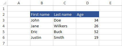
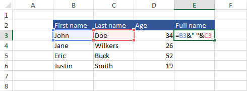
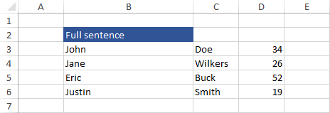
In the following example, we have a list of people. In the first column, there are first names, in the second- last names and in the third- ages.

Merging text

Create a new column, so you can place your merged data here. Name the cell E2 – Full name and then enter into cell E3 the following formula =B3&” “&C3 (this means: merge cell B3 with space and then with cell C3).

Press Ctrl + Enter to stay inside the cell. Move your mouse cursor over the bottom right corner of the cell. Use double-click to AutoFill names.

Suppose that after you created the Full name column, you don’t need the First name and the Last name columns anymore.

If you simply delete these columns, a reference error (=#REF!) will appear in the Full name cells. This error appears because these cells are not text values but rather references to columns B(First name) and C (Last name).

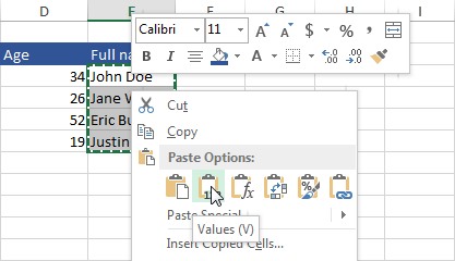
What you need to do is change the Full name cells to text values. Select cells from E3 to E6 and copy them Ctrl + C. Right-click on these cells and paste them as Values.

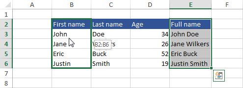
Select cells from E2 to E6 and move them into a place, where the First name cells are located.

Merging text with numbers

Delete the column Last name. Now you have columns with merged first names and last names.

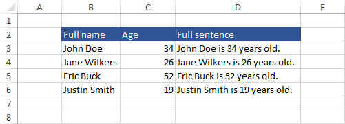
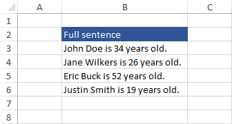
Let’s create a full sentence like “Full name” is “Age” years old. Enter formula =B3&” is “&C3&” years old.” into cell D3.

Use the AutoFill option to fill the rest of the cells.

Text to Columns Wizard in Excel 2016 Basics

In the previous lessons, you’ve learned how to merge data. In this lesson, you’ll learn quite the opposite. I will show you how to split data from a single column to multiple columns.

Example:

We will use the example from the previous lesson.

Convert Text to Columns Wizard

To split this data, first, you need to select cells from B3 to B6. Next, go to DATA >> Data Tools >> Text to Columns.

After the window Text to Columns Wizard will appear, choose the Delimited radio button.

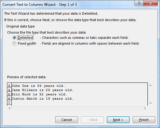
Click Next.

Because words in our example are separated by spaces, select the Space check box.

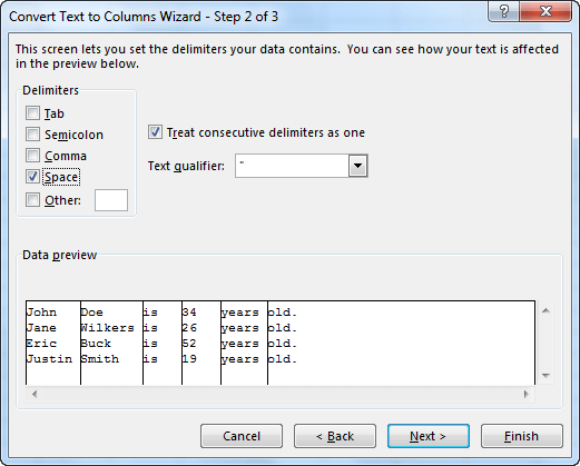
Click Next.

Click the third column and select the Do not import column (skip) option. Make the same changes for the fifth and sixth column.

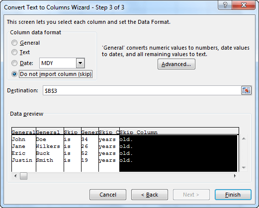
Click Finish.

Excel will split the data into three columns.

Change the headers to complete this example.

In next tutorial i will Write about Basics of excel 2016 like Finding and replacing data, Go to special, Naming cells and ranges, and Inserting rows and columns. Hope that it helps for you guys.