EXCEL 2016 interface Chapter 2

EXCEL 2016 interface Worksheets

Difference between a worksheet and a workbook

With EXCEL 2016 interface, you can achieve high efficiency with little effort. However, before you start working with the application, it’s good to know such basic things as the difference between a worksheet and a workbook.

EXCEL 2016 interface : Create Worksheet

A worksheet is a place where you can insert data, tables, charts, etc. In Excel 2013 a worksheet can contain up to 1 048 576 rows and 16 384 columns, which gives 17 billion cells.

Workbook

You can compare a workbook in Excel to the one you can find in the real world. It is a place where you can store your worksheets. An Excel workbook is a file that contains at least one visible worksheet.

In earlier versions of Excel, when you created a new file, the default workbook consisted of three worksheets. In Excel 2013 there is, by default, only one worksheet. Each additional, you have to add by clicking the plus icon, which is located to the right of the worksheet tab.

Worksheet operations

When you start creating additional tabs inside your workbook, you will notice that their default names and arrangement are not very intuitive. For that reason, you may want to make some modifications. Excel gives you that option. You can freely manipulate their names and location.

Below, you will find the list of operations that you can perform with Excel worksheets.

Adding worksheets

When you create a blank workbook, you will, by default, receive one sheet. If you want to add more sheets you can do it by clicking the plus button, which is located on the right side of the tabs.

Another way to add a new worksheet is to use the button in the ribbon. You can find it in HOME >> Cells >> Insert >> Insert Sheet. The difference between these two methods is that in the first one a worksheet is added to the right side of the active sheet, while in the second one to the left side.

Removing worksheets

Removing sheets is as easy as adding them, just right-click its tab and choose Delete.

You can also go to HOME >> Cells >> Delete >> Delete Sheet. If Excel finds that there is some data in the worksheet, it will display a message informing you that you won’t be able to restore it after you click the delete button.

Navigating between worksheets

You can navigate between worksheets in two ways. One of them is to click the tab of the sheet and the second one is to use Ctrl + PgUp and Ctrl + PgDn keyboard shortcuts.

Changing the worksheet position

To change the position of the worksheet, first, click (without releasing the mouse button) one of the tabs and then move it to the different location.

Notice that when you drag a tab, a small black triangle appears between two other tabs. It is showing you the location where the worksheet will be placed after you release the button.

Hiding worksheets

To hide the worksheet, right-click the sheet tab, then select Hide. If you want to show the hidden sheets, right-click any of the tabs and select Unhide. The window with a list of hidden sheets will appear. Choose which one you want to unhide and click OK.

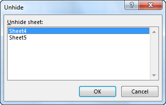
You can unhide only one worksheet at a time.

Renaming worksheets

Standard names that Excel assigns to worksheets are Sheet1, Sheet2, Sheet3, …. They are not very helpful when it comes to identifying their content. They become even less useful when you start adding more sheets, as their numbering does not necessarily reflect their position.

To change the name of the worksheet, right-click the tab and from the contextual menu select Rename. You can also do this by double-clicking the worksheet tab. Worksheet name then becomes editable.

CAUTION

If you try to enter the name “History”, a window with a warning message will inform you that this name is reserved for Excel.

Navigating inside the worksheet

Excel worksheet consists of columns (A to XFD) and rows (1 to 1 048 576). They form a grid that divides a worksheet into cells. Each cell has a unique address that is made of the column and row in which it is located. At one time, only one cell can be active- the one that takes the characters from the keyboard.

Look at the following example.

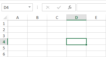
The active cell is in column D and row 4. It means that the address of the cell is D4 (it is shown in the upper left corner of the picture in the Name Box).

In Excel 2013, you can navigate through the worksheet not only with the mouse but also with the keyboard (and by touch on mobile devices).

Navigating with a mouse

To activate any cell, just click it. If the cell you want to activate is not visible on the screen, you can use the sliders to access it. You will find the slider (which let you scroll the page vertically) on the right side of the screen, and the other one (to scroll it horizontally) on the bottom right side.

Additionally, you can scroll the worksheet vertically using the wheel on your mouse.

Navigating with a keyboard

You can also navigate using the keyboard shortcuts.

↑ / Shift + Enter – move one position up.

↓ / Enter – move one position down.

← / Shift + Tab – move one position to the left.

→ / Tab – move one position to the right.

Ctrl + Enter – stay in the cell.

Ctrl + ← / Ctrl + → – move to the first/last element of the group of cells in the row. If you are in the last cell of the last group and you use the Ctrl + → keyboard shortcut, it will move the active cell to the last element in the row (XFD).

Ctrl + ↑ / Ctrl + ↓ – move to the top/bottom element of the group of cells in the column. If you are in the last cell of the last group and you use the Ctrl + ↓ keyboard shortcut, it will move the active cell to the last cell in the column (1 048 576).

PgUp / PgDn – go one screen up / down.

Alt + PgUp / Alt + PgDn – go one screen to the left / right.

Ctrl + Backspace – If the active cell is not visible, it moves the screen to show that cell.

Scroll Lock + Cursors – screen moves one step in the selected direction. At the same time, the position of the active cell doesn’t change.

Ribbon

The biggest change that has ever been done in the Office Suite user interface is the Ribbon. The first release of Excel that uses the Ribbon is Office 2007. It is also present in Office 2010 and Office 2013.

The idea behind the ribbon is to put there the most important features, so the user will have quick and easy access to them. It is divided into cards, which are divided into groups. Inside each group, there are tools and buttons thematically related to each other.

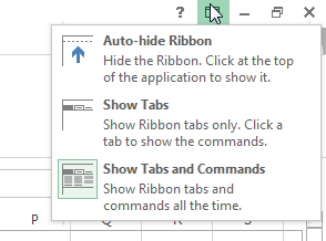
Hiding the Ribbon

If you need more space in the worksheet, you can increase it by collapsing the ribbon. There are two ways to do this:

1. Click the triangle-shaped button on the right side of the ribbon.

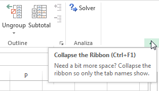
2. Use the Ctrl + F1 keyboard shortcut.

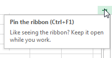
Showing the ribbon

There are two ways to show back the ribbon:

1. Use the Ctrl + F1 keyboard shortcut.
2. Click one of the tabs.

If you choose the second method you will also have to click the Pin the ribbon button. Otherwise, if you click anywhere outside the ribbon then it will collapse again.

You will find additional options in the upper right corner of the screen, next to the help button.

Ribbon tabs

The ribbon is divided into tabs. In each tab, you can find groups that are related to each other. Each group consists of features and buttons, which are designed for similar tasks. By using them, you can easily access the tool you are interested in, as well as explore other related features.

Excel tabs are divided into the following categories:

FILE

The FILE tab differs from the other tabs. In contrast to other tabs, it has been marked with a different color (for Excel- green). When you click it, it will take you to the Backstage view.

HOME

You will probably spend most of your time in Excel using this tab. It doesn’t contain features that are closely related to each other, but those that are the most popular and handy. Here, among other things you will find: formatting commands, text alignment, cell operations, searching, filtering and sorting data.

INSERT

Select this tab if you need to insert something in the worksheet. It can be a chart, table, picture, etc.

PAGE LAYOUT

This tab contains commands that will help you manipulate the look of your worksheet. Those tools are especially useful when you are planning to print your work.

FORMULAS

All functions that are available in Excel can be found in this tab. They are divided into categories, which you can access by clicking one of the buttons.

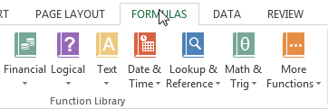
Here, you will also find a number of tools that will help you work with formulas. These tools are formula auditing or defining names.

DATA

With these tools, you can connect to an external data source, such as an SQL database. Tools such as sorting, filtering, and linking options will help you work with very large amounts of data.

REVIEW

This tab contains such tools as check spelling, add comments, translate words and protect worksheets.

VIEW

Here, you can enable or disable various display options. Some of them are also available in the Status bar.

DEVELOPER

This option is hidden by default. To unlock it, go to File >> Options >> Customize Ribbon and click the checkbox. It will add the Developer Tab to the ribbon. Now you will have access to options that can be useful for programmers.

Tool Tabs

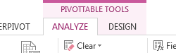
Tool Tabs contain additional tools. They appear right next to the main tabs. Depending on what you are currently working on, you will see different tools. For example, if you work with charts then they will look like this:

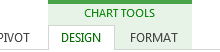
Tool tabs

In addition to cards that are, by default, displayed in the ribbon, there are additional cards that appear when you work with different things.

For example, if you work with images, the additional card, called PICTURE TOOLS will appear. It will help you work with images.

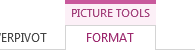
If you create a pivot table, then the PIVOTTABLE TOOLS will appear.

In order to view all available tool using one of the following methods:

1. Right-click any field in the ribbon and select Customize the Ribbon.
2. Go to FILE >> Options >> Customize Ribbon.

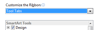
Under the Customize the Ribbon, in the upper right corner you will find a drop-down menu. Click it and select Tool Tabs. After you select this option, below the drop-down menu you will find all Tool Tabs that can be added to the Ribbon. You can expand them and explore their contents.

How to customize the ribbon

The Ribbon is designed to help you achieve greater productivity in Excel. It can be customized to meet your individual needs.

To open the Customize the Ribbon window, do one of the following:

1. Go to FILE >> Options >> Customize Ribbon.
2. Right-click any field in the ribbon and select Customize Ribbon.

A new window will appear.

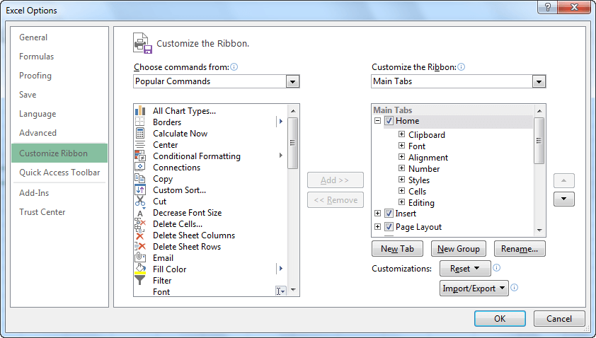
On the right side of the window, you will find items with checkboxes that represent tabs in the ribbon. You can select or deselect them, depending on whether you want the tab to be visible in the ribbon. Expand the tab to see what groups it is composed of. Expand the group to get access to its elements.

Creating a new tab

Another thing you can do with the ribbon (in addition to hiding and displaying its elements), is creating your own tabs. To create a new tab, click the New Tab button.

After you click the box, on the right side you will see a new item, named New Tab (Custom). It includes a group called  New Group (Custom).

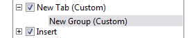
If you want to change the name of the new tab or group, right-click it and choose Rename. Alternatively, you can choose to click the Rename button, which is located below the tabs. In the window that appeared, enter a new name. Notice that when you change the group name, you will have a further opportunity to select the corresponding icon that will be displayed in the tab.

After you change the names of the buttons, Excel leaves text “(Custom)” at the end of the name. The application does this, so you won’t forget that the tabs have been created by you and are not Excel default tabs.

To add new items, first click that group, then start adding options and features which you want to be present in the Tab.

Additionally, if you don’t like the position of the tab, you can use the buttons that are located on the right side of the window.

Resetting the ribbon

If you want to go back to the previous settings, click the Reset button. Here, you will find two options.

Reset only the selected ribbon tab

You can use it if you made changes inside one of the default Excel tabs.

Reset all customizations

Undo all changes and restores the ribbon to its original state.

Using the keyboard to work with the Ribbon

If you think that working with Excel with a keyboard is more convenient than with a mouse, you will probably be happy that the individual elements of the ribbon can also be controlled by the keyboard.

If you want to access the ribbon by using the keyboard, press the left Alt keyboard shortcut.

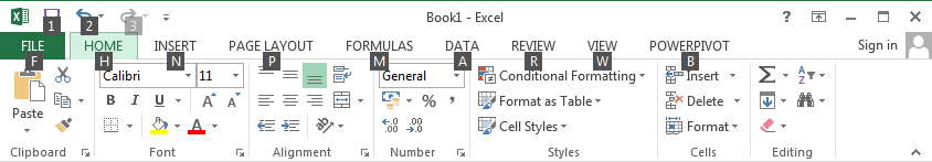
Excel will display icons thanks to which, you know which part of the ribbon corresponds to which character. Here, unlike the keyboard shortcuts, you don’t hold two keys at the same time but press them one after another.

Example:

Suppose that you want to change the font size for the values in the selected cell. The first thing you need to do after pressing the Alt key is to select the Tab you are interested in.

Press the key which is assigned to the tab, even if the tab is currently opened. In our case, press the h button to select the HOME tab. Next, you will get another set of characters. This time, you can select options and features inside the previously selected Tab.

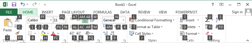
To select the font size, first press “f” and then “s”.

Enter the font size you want and confirm with the Enter key.

TIP

If you want to return to the previous selection, press the Esc key.

In next tutorial i will Write about Interface like Quick Access Toolbar, Formula Bar, Status Bar and Backstage View. Hope that it helps for you guys.