Excel 2016 Basics Chapter 8

In this tutorial i will cover Basics of excel 2016 like Color, type and font size, Bold, italic, underline, and strikethrough, Filling cells, and Cell borders.

Color, type and font size

If you want to change the look of the worksheet, you can do it in a very simple way- by changing the type, size or font color.

Excel has an interesting feature to automatically change the appearance of a cell and text formatting after you hover your mouse cursor over one of its predefined styles. With this quick preview, you can check how your text will look like if you apply the changes.

Type and size

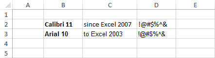
The default font since Excel 2007 is Calibri, size 11. In Excel 2003 and earlier versions, it was Arial 10.

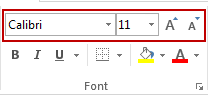
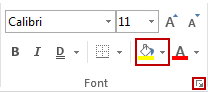
To change the font size, go to HOME >> Font. In the upper left corner of the font area, you will find information about the font that was used in the text. If you want to use another one, click the small triangle on the right side of the font name to expand the list of fonts and choose one of them.

On the right side of the font name, you will find the font size drop-down. You can expand the list of sizes or just enter a new one from the keyboard.

On the right side of the font sizes, you can find two icons- the first one is used to increase and the second one to decrease the font size.

Color

If you want to change the font color, go to HOME >> Font >> Font Color. Here, you will find the most popular colors and their shades.

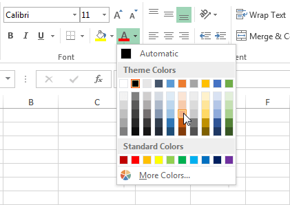
If you don’t find any color that suits your needs, click the More Colors position. A new window will appear. It is divided into two tabs. One of them is the Standard tab, which contains a set of standard colors.

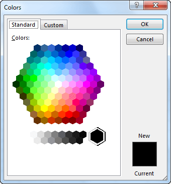
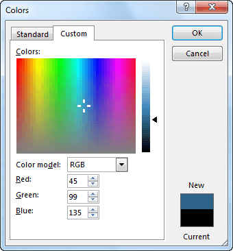
It will give you access to 127 colors and several shades of gray. If you are still not satisfied with the number of colors, click the Custom tab. Here, you can create your own colors by changing the intensity of the three primary colors: red, green and blue. It will give you a total of over 16 million combinations.

Bold, italic, underline, and strikethrough

Besides changing the color, size and font type, you can highlight text in Excel in several different ways. For example, using: bold (Ctrl + B), italic (Ctrl + I), underline (Ctrl + U), and strikethrough.

Bold and italic

Many fonts have a few different variations, such as regular, bold and italic. If a font has only a regular type, then Excel creates the other two by using its own algorithm.

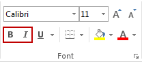
You can find the bold and italic buttons in HOME >> Font.

You can combine them or use them separately. As a result, the text can be written in italics, bold, or bold italics.

Underline

You will find the underline button on the right side of the bold and italic buttons.

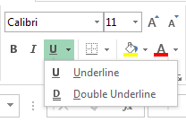
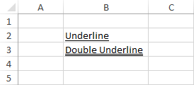
When you click the triangle you will have a choice whether you want your text to be Underlined or Double Underlined.

In addition to the standard underline, you can also use the Accounting Underline. You won’t find it directly in the ribbon, so you have to click the little square icon in the lower right corner of the font group.

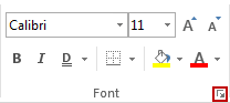
You can also use the Ctrl + Shift + F keyboard shortcut.

When a new window opens, select from the drop-down list the Single Accounting or Double Accounting underline.

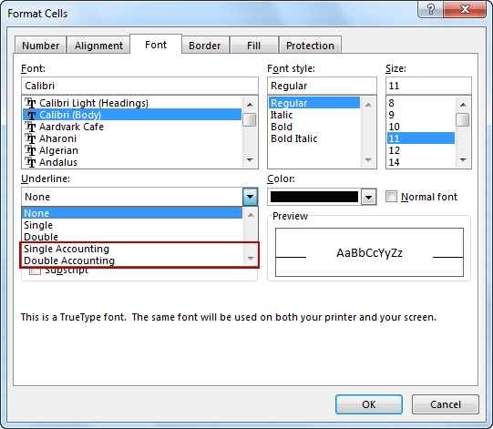
There are two differences between the standard underline and the accounting underline:

1. In the accounting underline, the whole text is placed above the line. In the standard underline parts of some letters can be under the line.
2. In the accounting underline, the line is stretched across the width of the cell, while in the standard underline the width of the line is equal to the width of the text.

Strikethrough

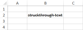
In order to use the strikethrough, select text and use the Ctrl + Shift + F keyboard shortcut.

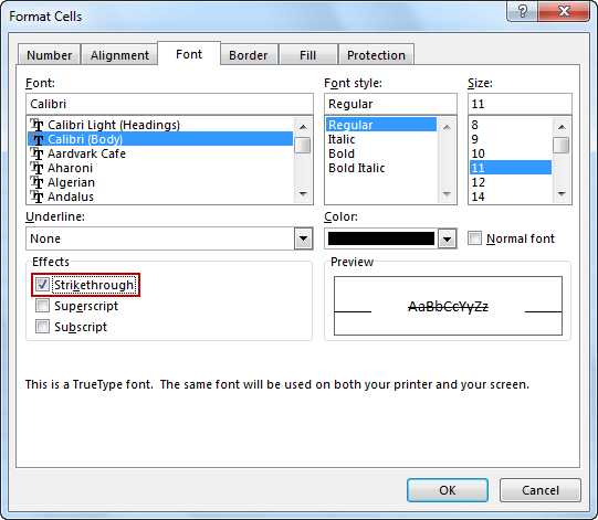
In the Effects area check strikethrough, click OK and see the effect.

Filling cells

Besides text formatting, you can also highlight particular cells by changing their background type. In Excel, you can fill cells with color, gradient, and pattern.

Example:

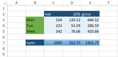
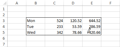
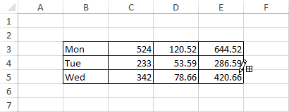
Look at the following example. It shows our expenses for the next three days.

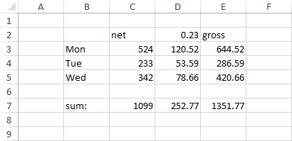
It is a “clean”, unformatted example, which is not very legible. Let’s format some of the cells to create a nicer look.

The Fill icon is located in HOME >> Font >> Fill Color. There is an additional icon in the lower right corner. Click it and you will get access to additional options.

Filling cells with solid colors

Select cells from B3 to B5. From the drop-down menu select the color Green, Accent 6. Then select cells from C2 to E2 and cell B7. Fill them with Blue, Accent 1, Darker 50%.

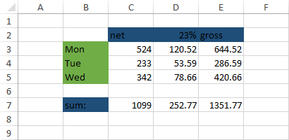
For the cells with the dark blue background choose a white font color to make the text more readable. The Font Color icon is located next to the Fill Color icon.

Filling with gradient

As I wrote at the beginning of this lesson, instead of using a solid color to fill the cell background, you can also use a gradient.

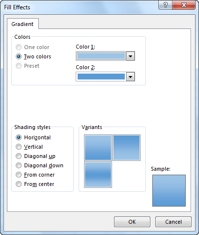
To do it, first select cells from C7 to E7. Right-click them, and then select Format Cells… or use the Ctrl + Shift + F keyboard shortcut. When a window opens, select the Fill Effects… button.

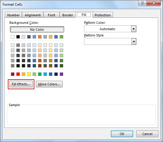
In the new window, you can set two colors. I suggest that you choose colors that are similar because the transition between them will be more subtle and it will create a more professional look.

Filling cells with a pattern

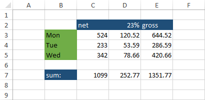
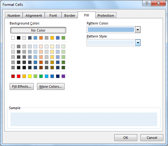
Select cells from C3 to E5. Open the Format Cells window and then click the Fill tab. On the right side, you will find two drop-down menus: Pattern Color and Pattern Style. I suggest that you choose a light color, otherwise the background pattern will be distracting.

After you confirm changes, the pattern will be applied to the cell. Now, the example looks much better than at the beginning and is also more readable.

Removing fill

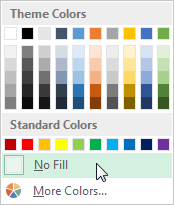
If you want to remove the fill from the cells, choosing a white background is not the solution here, because it will also remove the grid separating the cells from each other. Besides, it won’t remove the pattern fill.

What you should do is use the No Fill option. You can find it in HOME >> Font >> Fill Color >> No Fill.

Cell borders

Besides changing the font and color of cells, you can also distinguish them by using cell borders.

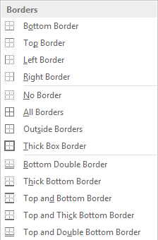
In order to add borders, go to HOME >> Font >> Borders.

When you expand the Borders button, you can find many different options, such as Outside Borders, Thick Borders, All Borders, etc.

Below this list, you can find options to draw and erase borders or set line color and style.

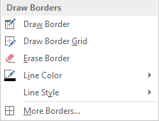
If you want to draw a border manually, click the Draw Border button and select the cells that you want to have borders.

To create a border grid, select the Draw Border Grid button.

If you want to erase borders, use the Erase Border button, then choose the cells from which you want to remove them.

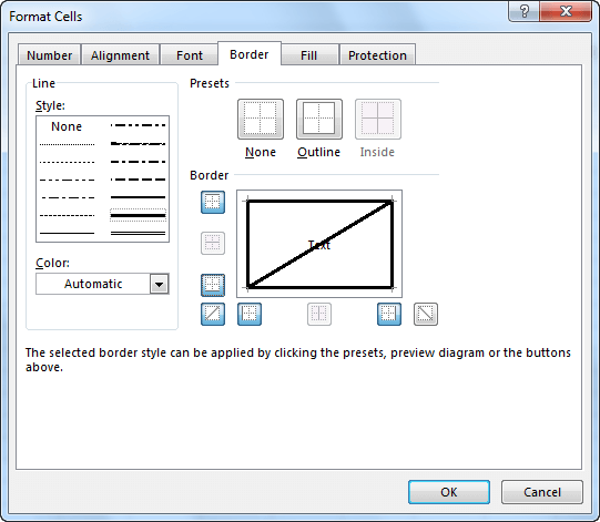
If you need more options, select the More Borders… button. A new window will appear. Here, you can change the border type, border color and select the edge of the cells to which you want to apply your border.

Besides borders, you can also use a diagonal strikethrough from top-left to bottom-right and from bottom-left to top-right.

In next tutorial i will Write about Basics of excel 2016 like Simple fractions and decimal fractions, Currency and accounting format, Custom number formatting and How Excel stores date and time. Hope that it helps for you guys.