EXCEL 2016 interface chapter 1

Start Screen of excel 2016 interface

When you start Excel 2013, the program displays the default startup screen of excel 2016 interface, similar to the one displayed in the following image.

Excel 2016 interface or Startup Screen is divided into two panels:

Left panel

Here, you will find a list of recently opened files and the button called Open Other workbooks, which is located at the bottom of the panel. from here we can open recent file or other workbooks if we want.

Right Panel

The Right panel shows a list of default templates that are available in Excel.

If none of them meets your expectations, you can use the search bar by typing the phrase you want. In this case, Excel will be searching for templates that are available on the Internet.

Additionally, below the bar, you will find some of the most popular phrases. When you click one of them, Excel will start searching for templates in this category.

Creating a new document

To create a new document in excel 2016 interface, click the first item called the Blank Workbook. You can also do this by using the Ctrl + N keyboard shortcut, On the File tab, click New. or In the Search online templates box, enter the type of document you want to create and press ENTER.

TIP

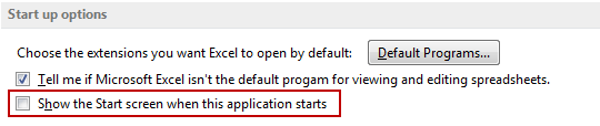
For the first time, EXCEL 2016 interface or the startup screen appeared in Excel 2013 and is, by default, displayed when you start the program. If you want to see a Blank workbook instead, go to File >> Options >> General and uncheck the Show the start screen when the application starts checkbox. like picture shown below;

EXCEL 2016 interface : Application window

With Excel 2007 Microsoft introduced a revolutionary new look for the Office Suite applications. The major change was the Ribbon, which completely changed the way we use Excel and other Microsoft Office applications.

The major change was the Ribbon, which completely changed the way we use Excel and other Microsoft Office applications.

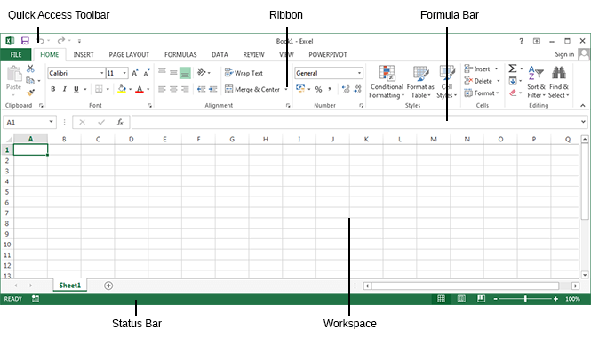
Below, I described different parts of Excel 2013. Please take a look.

Quick Access Toolbar

The Quick Access Toolbar is a customizable toolbar that contains a set of commands that are independent of the tab on the ribbon that is currently displayed. You can move the Quick Access Toolbar from one of the two possible locations, and you can add buttons that represent commands to the Quick Access Toolbar. This is the last “real” toolbar that you can still find in Excel 2013. It’s a place where you can put the most frequently used Excel commands.

The Quick Access Toolbar can be located above or below the ribbon. Contrary to the earlier releases, in Excel 2013 Microsoft abandoned the possibility of attaching it to the side of the screen.

Ribbon

Options in Excel 2003 that were available in the drop-down toolbars have been moved to the ribbon. This allows you to find them easily because they are thematically arranged on the tabs, which are then divided into groups.

Formula bar

It’s located below the ribbon. In the formula bar, you can find the content of the currently selected cell. You can also enter and edit data inside the formula bar.

Workspace

The working area is divided into cells, rows, and columns. The address of the cell is determined by the row and column where it is located. For example, if a cell is placed in column K and row 5, the address of the cell is K5.

Status bar

The status bar informs you about the current state of the worksheet. Here, you will also find icons that are responsible for zooming the working area.

In next tutorial i will Write about Interface like Worksheets and Ribbon. Hope that it helps for you guys.