Excel 2016 Basics Chapter 3

Excel 2016 Basics Flash Fill

Flash Fill is a tool available in Excel 2016 Basics that is similar to AutoFill and Text to columns.

In contrast to AutoFill, Flash Fill is not restricted to a single row or column, but it also looks at the surrounding cells to find more complicated patterns.

It differs from the Text to columns tool in that, it can extract numbers that are separated by different delimiters and can also be located in different positions inside the cell.

You can find Flash Fill in three different places:

1. HOME >> Editing >> Fill >> Flash Fill,
2. DATA >> Data Tools >> Flash Fill,
3. Ctrl + E keyboard shortcut.

Example 1:

Let’s use the following example.

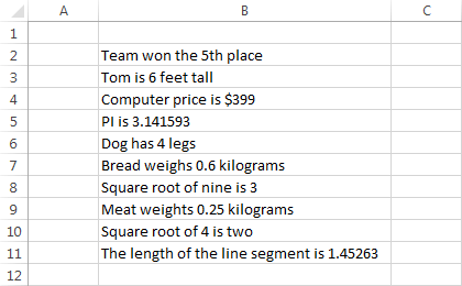
Suppose that you want to extract the number from each cell and insert it into the cell in the right column.

Not all of them are separated by space (e.g. $399) and they are located in different places. This is a perfect example to demonstrate how the Flash Fill works.

Enter number 5 in cell C2 and press Ctrl + Enter to stay inside the cell. Use Flash Fill to fill other cells.

Notice that the data inside cells C5, C7, C9, C11 doesn’t contain decimal fractions but integers. Now, change the value 141593 in cell C5 to value 3.141593.

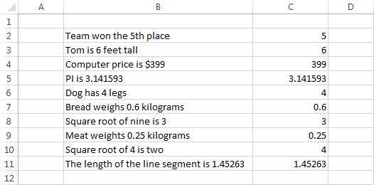
Look that the Flash Fill tool „learns” from your corrections, so it is very important for the data to be consistent.

Excel 2016 Basics Spell checking

Spell checking is well known to those who work with text editors, such as Microsoft Word.

Because you use text not only in text editors, spell checking can also be useful in other programs. That’s why Microsoft added this tool to other Office applications.

To open the spell checker, select REVIEW >> Proofing >> Spelling or use the F7 key. Excel checks the spelling cell by cell, row by row. If it encounters value that seems to him to be incorrect, it stops there and displays a list of suggestions where you can decide what you want to do in the current situation.

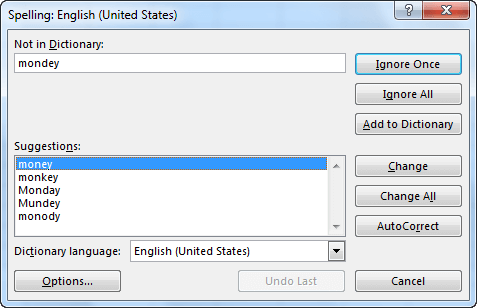
If Excel doesn’t encounter any suspicious words it displays the message informing you that the spell checking is complete.

Excel 2016 Basics Undo and Redo

When you work with a worksheet, Excel records every change you make. For example changes in cells, cell and text formatting, cutting, copying, pasting, editing, etc.

Excel can successfully save up to 100 changes, without slowing down the computer.

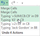
You can control these changes by using two commands located in the Quick Access Toolbar: Undo and Redo.

If you want to go back to the particular state, click the triangle next to the Undo icon, then choose a position you want to go back to. The changes are described, so you can go back to the exact state, without guessing.

The Redo icon becomes active when you go back at least one position. With Redo as well as with Undo you can click the triangle (that is located in the same button) and select an item from the list.

TIP

Instead of clicking the arrows, you can also use the Undo (Ctrl + Z) and Redo (Ctrl + Y) keyboard shortcuts.

CAUTION

Some actions cannot be undone. One of them is removing a worksheet from the workbook.

Excel 2016 Basics Hyperlinks

A Hyperlink is a text, which references to a particular place. It is usually highlighted and underlined in a way that it can be distinguished visually from normal text. You often deal with hyperlinks when you view web pages. But you can also find them in Excel and they have a similar purpose to those found on web pages.

To insert a new hyperlink, go to INSERT >> Links >> Hyperlink. After you click the button, note that on the left side there are four different buttons, which you can use to insert hyperlinks.

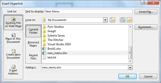
Excel 2016 Basics : Existing file or web page

You can create the hyperlink that points to a website (which will open in a browser) or a file (which will be opened by the default program).

The text of the hyperlink will be the name of the file or the page address you entered. To change this, click the text box, which is located next to the Text to display.

Click the OK button to insert the hyperlink.

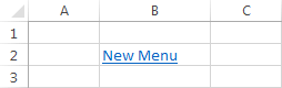
When you click the link, it will be opened by the default browser or default application, depending on whether you entered a website address or a link to a file.

TIP

By default, Excel converts text to link when you enter the address of a website directly into a cell or the formula bar (for example „http://google.com” or „www.google.com”). If you want to enter a web address as a text, use the Ctrl + Z keyboard shortcut, just after you confirm the entered value.

Excel 2016 Basics : Place in this document

The second button is the button called Place in This Document. It is used to insert a reference to cells which are located in the worksheet.

If you have multiple worksheets in the workbook and you want to place the hyperlink that points to a different worksheet, you can do it by selecting it from the list.

Excel 2016 Basics : Create a new document

At this point, Excel allows you to create a hyperlink to a document. The document is automatically created after you click the OK button.

Here, you can choose whether a new file should be opened for editing or saved as a blank document.

Excel 2016 Basics : E-mail address

When you click this link you can send an e-mail. If your mail client is not configured then a message will inform you that you cannot perform this operation.

TIP

If you want to quickly insert the hyperlink, press Ctrl + K shortcut.

Excel 2016 Basics Data validation

There may be situations when you want to prevent users from entering data that doesn’t meet the conditions you specified.

Suppose that you have the cell in your worksheet where you want a user to enter his age. Therefore, as a condition, you require the integer between 18 and 99.

To set a condition, first, select the cell or the range of cells, then click DATA >> Data Tools >> Data Validation. After you do that, a new window will appear.

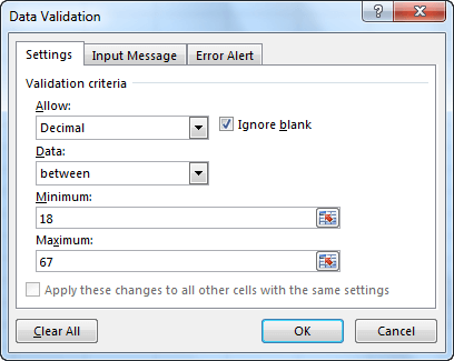
Settings

Here, you can specify which kind of data and range you want to set for the selected cells.

You can use one of the following data types:

Whole number

Numbers that are not fractions (-12, 0, 4, etc.).

Decimal

These numbers can also be fractions (1.2, -1, 5, 4.6, etc.).

List

With this type of validation, you can choose from the drop-down menu one of the several items.

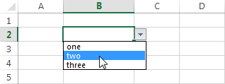
If you choose List, the new textbox, called Source will appear. In this textbox, you can select cells from the worksheet or enter values from the keyboard- for example “one,two,three” (or “one;two;three” depending on your system configuration).

Date

Here, you can enter date and time. (“3/14/2014”, “14-Mar”, “14”).

CAUTION

If you enter a date without a year- for example, “14 March”, Excel will treat this record as “13 March 2014” (current year). If you enter only a day, for example, “14”, it might seem that it is a day of the current month and current year. However, in this case, it will be regarded as “14 January 1900”. That’s because the text “March 14” is treated as a date and “14” as a number. You will learn more about dates in future lessons.

Time

Here, you can enter an hour. For example: “12:00”, “1:14:50 p.m.”.

TIP

If you want to see which date and time formats you can use, right-click the selected cell and choose Format Cells…. After you click the position from the category on the left side, a list of different formatting options will appear.

Text length

Here, you can specify the number of characters that must be entered. You can enter plain text, as well as numbers.

CAUTION

There may be some confusion when you deal with dates. If you set the length of the text range for 3 to 5 characters, and then you enter the date “March 14, 2014” (14 characters), format it to “14-Mar-14” (9 characters) Excel won’t return an error. That’s because a date in Excel is stored as a number and is only formatted as text. If you want to see that number, right-click this cell and select Format Cells … from the contextual menu. Select Number and click OK. As you can see this number is “41712”. It consists of 5 characters, which are inside the specified range, so this number won’t return the error.

Custom

Custom validation is more complicated than other types of validation. Here, you can insert a formula with the specific parameters.

At the bottom of the window, you will find the checkbox called Apply this changes to all other cells with the same settings. It means that if you click the cell and select this option, Excel will check in a worksheet (not a workbook) whether there are other cells with the same validation parameters. If so, all these cells will be selected and the changes applied.

Input Message

Here, you can set a pop-up window with a title and input message. Now, when you click the cell, a window with an entered message will appear.

Excel 2016 Basics : Error Alert

Stop

Excel displays an error message with the Retry and Cancel buttons. If you select the Retry button you’ll get a chance to re-enter the value. If you choose the Cancel button, the value will be restored to the one that was previously entered.

Warning

In this case, Excel displays a warning message. There are three options available: Yes, No and Cancel. If you choose Yes, Excel will enter the value that doesn’t meet the conditions. If you click No, Excel will let you change the data. If you click Cancel then the data will be restored to the previous value.

Information

When information window appears, you can click OK to accept the value or Cancel to return to the previous state.

CAUTION

Excel checks the value only after you create the validation rule. If you apply validation to the cells that already contain values, Excel will not complain, even if those values are incompatible with the rule.

Excel 2016 Basics : Removing validation

If you want to remove the validation from the cells, first select these cells, then click the Clear All button in the lower left corner of the Settings tab. Click OK to confirm.

In next tutorial i will Write about Basics of excel 2016 like Comments, Selecting cells, Select rows and columns, and Inserting cells. Hope that it helps for you guys.