Excel 2016 Basics Chapter 4

Comments in Excel 2016 Basics

Comments in Excel can be used to describe different cells in a worksheet, without changing their contents. Excel 2016 Basics You can use comments in many different situations, such as: asking a question, drawing attention or informing about a mistake.

Inserting comments

There are three different ways you can use to add comments in Excel 2013:

1. REVIEW >> Comments >> New Comment.
2. Right-click a cell and choose Insert Comment.
3. Use the Shift + F2 keyboard shortcut.

After you choose one of these methods, Excel will insert a new box. At the top of it, you will find your name (which you can delete) and the place to insert your text.

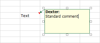
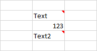
To exit the edit mode, click any cell or press the Esc key twice. The Cell containing a comment will be marked with a small red triangle in the upper right corner.

Editing comments

If you want to edit a comment that already exists, go to REVIEW >> Comments >> Edit Comment or use the Shift + F2 keyboard shortcut.

Showing and hiding comments

In order to preview comment, hover your cursor over the cell that contains a comment.  If you want comments to be constantly visible, go to REVIEW >> Comments >> Show/Hide Comment. In order to do the same for all comments at once, choose the Show All Comments button.

Select cells in Excel 2016 Basics

Excel allows you to select cells in several different ways, using both the mouse and the keyboard.

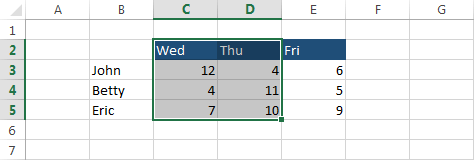
Selecting with a mouse by dragging

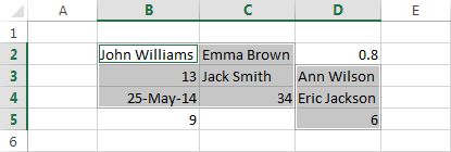
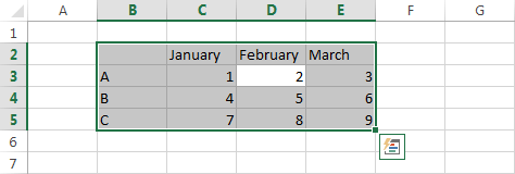
Look at the following example. It contains 16 cells filled with data. To select them, click cell B2 and drag the cursor to cell E5. After you release the mouse button the cells will be selected. You can start selecting them from any corner of the table.

Selecting cells by using the Shift key

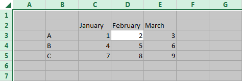
In the second method of selecting data, we will use the Shift key. In this case, click any corner of the table, then, while holding down the Shift key, click the opposite corner.

Selecting cells with the Ctrl + A keyboard shortcut

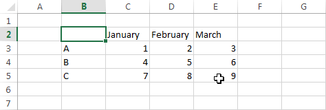
To use the third method, click any cell that is located in the table, then use the Ctrl + A keyboard shortcut.

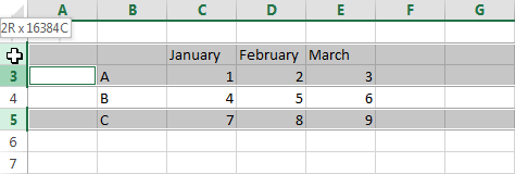
Selecting the entire worksheet with the Ctrl + A keyboard shortcut

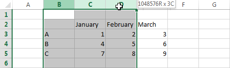
To select all cells in a worksheet, use Ctrl + A twice or click the icon in the upper-left corner of the worksheet.

Selecting non-adjacent cells

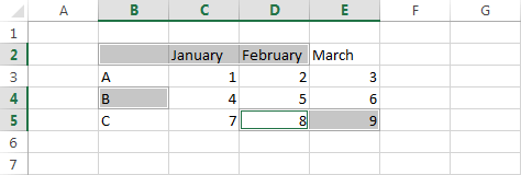
If you want to choose non-adjacent cells, click or click and drag different cells while holding down the Ctrl key.

Selecting rows and columns in Excel 2016 Basics

In the previous lesson, I presented a few ways to select cells and ranges. This time, I will show you a few methods for selecting columns and rows.

Selecting with mouse

To select multiple columns at once, click one of the letters at the top of the worksheet area and without releasing the mouse button, drag it to the right or left. In the same way, you can also select rows.

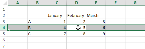
Selecting non-adjacent rows or columns

If you want to select multiple non-adjacent rows, you can do this by clicking the rows’ numbers while holding down the Ctrl key.

Using keyboard shortcuts to select rows and columns

You can also select rows or columns by using the keyboard shortcuts. Use Shift + Space to select the entire row and Ctrl + Space to select the entire column.

Inserting cells in Excel 2016 Basics

Sooner or later you will need to insert additional cells between those that already contain data. Of course, you can move the contents of those cells to make a place for new data, but there is another faster method, which I will show you in the following example.

Example 1:

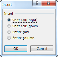
To insert the cells inside a worksheet, first select a place where you want to put them, then right-click the selection and choose Insert.

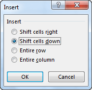
When you choose this option, a window with four radio buttons will appear. By default, Excel sets the option, which it considers the most likely in this case. In our example, the default option- Shift cells right is the option we want.

After the cells are shifted to the right, new blank cells appear in the table.

Example 2:

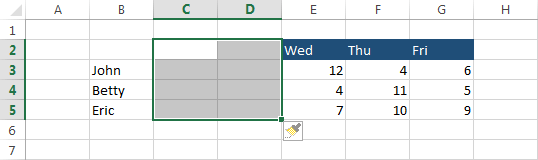
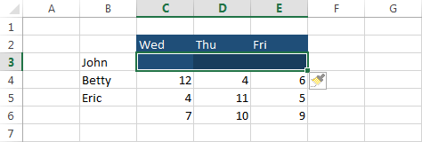
In the second example, we will insert new cells below the table header. Select cells from C3 to E3. Right-click them and select Insert. This time, Excel also guessed correctly. We want the cells to be shifted down.

Newly inserted cells will inherit the cell formatting from the cells that are located above or from those to the left, depending on where you want to insert the new ones.

In next tutorial i will Write about Basics of excel 2016 like Cell references, Merging cells, Merging text with numbers, and Text to Columns Wizard. Hope that it helps for you guys.