Excel 2016 Basics Chapter 2

Windows and Office Clipboard

Excel 2016 Basics : Windows Clipboard

The Windows Clipboard is a place where the most recently cut or copied value is stored. This can be a value from Excel 2016 basics or any other Windows application. For example, you can copy a value from a web browser and paste it into a Notepad, Word, Excel, etc.

Each clipboard value is replaced by the next one that is copied or cut because the Windows Clipboard stores a single value at a time.

Excel 2016 Basics : Office Clipboard

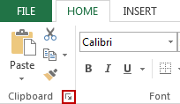
Similarly to the Windows clipboard, the Office Clipboard stores only one- last copied or cut value. If you need Excel to remember more than a single value, click the button in the HOME >> Clipboard group.

The Office Clipboard will appear on the left side. Start copying cell contents, and they will appear automatically on the clipboard list.

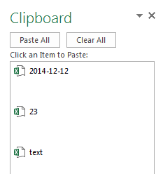
If you want to insert one of those values, select the cell where you want the value to be pasted and click the value from the clipboard. You can paste all values at once by using the Paste All button. If you want to get rid of the contents of the clipboard, click Clear All.

TIP

The values stored in the Office Clipboard in one application can be accessed by other Microsoft Office applications. For example, if you copy the contents of a cell in Excel, then it will also be available in Word and vice versa.

Excel 2016 Basics : Paste Special

In addition to the standard data pasting, Excel allows you to paste data in a special way. Unlike normal pasting, in Paste Special you have more control over how the pasted content will look like. The Paste Special works only when you copy (not cut) the contents of a cell.

In order to use the Paste Special feature, copy the contents of the selected cells and choose a place where you want to paste these values. Use the right-click to open the contextual menu.

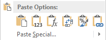
Here, you will find the most popular options for pasting. If none of them meets your needs, you can click the triangle on the right side of Paste Special to display additional options.

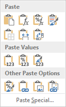
The paste options are divided into three groups: Paste, Paste values, and Other Paste Options.

Paste

Paste (P)

This is the standard method for pasting data. It has the same effect as using the Ctrl + V keyboard shortcut.

Formulas (F)

In this case, Excel remembers that the pasted data has to be treated as a formula. Sometimes when you open more than one instance of Excel and then you use the standard paste method (Ctrl + V), it might be treated as an ordinary value. Therefore, in such cases, it is safer to use Copy as Formula.

Formulas & Number Formatting (O)

In this pasting method, the pasted value keeps the format. For example, 4.0934% is pasted as 4.0934% and not, for example as 4.09%.

Keep Source Formatting (K)

This method is similar to the one above. The difference is that this method also copies such changes as font and background formatting.

No Borders (B)

If you copy from the cell with borders and then you paste the data to another cell, all the formatting but borders are copied.

Keep Source Column Widths (W)

Pastes cells in the same way as the Keep Source Formatting method. The only difference is that it copies also the width of the column.

Transpose (T)

You can use this method if you want to switch columns and rows.

Paste Values

Values (V)

Let’s suppose that the cell displays value 6, but, in fact, this is the formula (=2+1+3). With this type of pasting the value 6, not the formula is copied.

If you enter 4.0954% + 1% then the displayed text will be 5.10% (rounded 5.0954%). Paste this value using the Values method and it will be displayed as 0.050954.

Values & Number Formatting (A)

Let’s use the formula from the previous example (=4.0954% + 1%). In this case, the formatting will be preserved. However, it won’t be remembered as a formula, but as value 5.0954%.

Values & Source Formatting (E)

This pasting method is similar to Values & Number Formatting, with the difference that it also preserves cell formatting.

Other Paste Options

Formatting (R)

In this case, we don’t copy the cell value, but its formatting (background color, size, font color, etc.).

Paste Link (N)

This method pastes a link to the copied cell. If you copy cell A1 to B1, then cell B1 will contain a link to cell A1 (=$A$1). That means, that when you change the contents of cell A1, the contents of cell B2 will change automatically. In this case, the formatting is not preserved.

Picture (U)

Pastes the contents of a cell together with formatting and saves it as a picture. Here, you can perform the same operations as on any other image.

Linked Picture (I)

Similar to the previous example it pastes contents as a picture. This time, however, the picture is linked to the copied cell and, therefore, it is updated every time you change the contents of the cell.

The Paste Special button

If you need more options, click the Paste Special button.

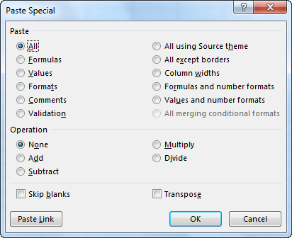
Here, you will find such features as automatic addition, subtraction, division or multiplication. Additionally, you can copy the only width of a column or its validation.

Excel 2016 Basics : AutoCorrect

As soon as you start typing text in your worksheet, the Excel AutoCorrect feature monitors every move you make and corrects minor errors, such as typos or lower and upper cases.

Example:

If you type the word “HEllo”, it will be automatically converted to the word “Hello”.

If you want to enter the word starting with a capital letter, but there was the Caps Lock key pressed, then the text “hELLO” will be changed to “Hello” and the Caps Lock key will automatically turn off.

AutoCorrect settings

The AutoCorrect feature can be adjusted in FILE >> Options >> Proofing >> AutoCorrect. You can select in which cases you want Excel to assist you when you typing. Here, you will find a list of words with the most common typos. You can either delete them or add the new ones.

Using AutoCorrect feature to create shortcuts

Note that you can use the AutoCorrect feature, not only to correct words but also to create abbreviations. For example, the notation “(c)” is automatically changed to “©”.

Let’s suppose that you want to create your own shortcut. For example, the phrase “to be continued”, which will be displayed when you type the word “tbc”.

In order to create it, go to FILE >> Options >> Proofing >> AutoCorrect Options. Then in the Replace textbox enter the abbreviated form “tbc”, and in the With textbox enter “to be continued”.

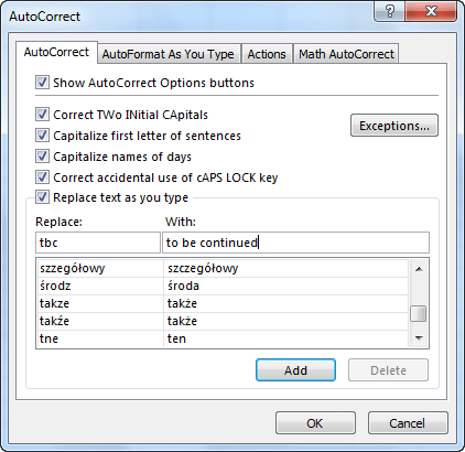
Now, each time you type text “tbc”, it will be replaced with “to be continued”.

NOTICE

The AutoCorrect works between all Microsoft Office applications.

Excel 2016 Basics : AutoComplete

When you work with worksheets, sometimes you will need to enter the same text multiple times. To automate this task, Microsoft introduced the AutoComplete feature.

To better illustrate how this tool works, take a look at the following example:

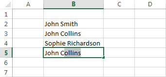
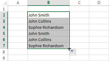
Here, you can see that name “John Smith” appears in cell B2. The Name “John Collins” in cell B3 and the name “Sophie Richardson” in cell B4. As soon as you start typing, Excel compares your input to the cells located above.

When you type the first letter “J”, Excel won’t give you any hints, because it doesn’t know whether you mean “John Smith” or “John Collins” or maybe a completely different name.

But when you type “John C” Excel will “know” that there is a good chance that you meant “John Collins”, because there is no other “John”, whose last name begins with the letter “C”.

If the text suggested by Excel is the one you want, you can go to the next cell, but if you meant a different one, then continue typing until Excel guesses what you are looking for.

Limitations of AutoComplete

The AutoComplete feature has several limitations:

• It only works with text. It doesn’t work with numbers and dates.
• It doesn’t check the data in other columns than those located above.
• If there is a break in the form of an empty field between typed text and the values above, then Excel will treat it as another list, even though it is in the same column.

AutoComplete Options

If you want to disable AutoComplete, you can do it in FILE >> Options >> Advanced >> Editing Options >> Enable AutoComplete for cell values.

Excel 2016 Basics : AutoFill

AutoFill is a very useful Excel feature. It allows you to create entire columns or rows of data which are based on the values from other cells. In other words, Excel compares the selected data and tries to guess the next values that will be inserted.

AutoFill months and days

Example 1:

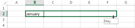
Look at the following example. In cell B2, there is the word- “January”. Excel automatically recognizes it as the first month. Click this cell to activate it. Move the cursor to the bottom right corner so that it will change to a small black cross.

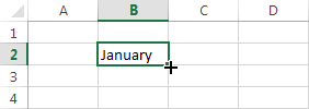
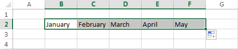
Drag your cursor to cell F2. As long as you hold down the mouse button, Excel shows you which month will be inserted into the last cell in a small rectangle.

TIP

AutoFill works both vertically and horizontally

Release the key to insert the values into the cells.

Example 2:

You can use AutoFill, starting from any list item- not necessarily the first. See how it works in the following example, with days of the week.

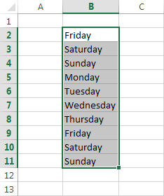
Notice that when the list reaches the end, Excel starts to insert new elements, starting from the beginning of the list.

AutoFill numbers

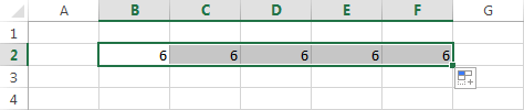
Auto filling numbers is slightly different than filling data that is saved in the defined lists. If you put a number and use the AutoFill feature, Excel will fill all selected cells with the same value.

If you want each next number to be incremented by one- compared to the previous one, you can perform the same operation as before, but this time holding down the Ctrl key.

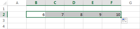
You can also use AutoFill to insert lists of odd and even numbers, tens, etc. In this case, you must select at least two cells with the values.

CAUTION

Unfortunately, Excel 2016 Basics can handle only simple examples. If you have more complex ones, the result probably won’t be the one you expected. So be careful when you use this feature.

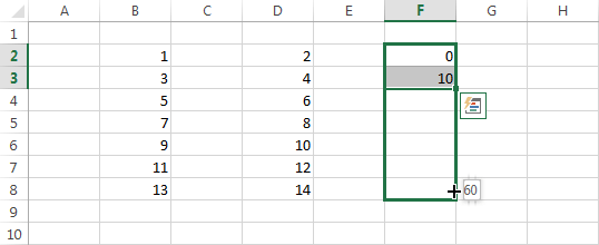
Example:

Look at the following example. Suppose that you want each next number to be the sum of all the previous. You entered the following values: 1, 1, 2, 4, 8, 16.

If you select these values and use the AutoFill feature to fill the other cells, you will see that Excel has treated them in a completely different way.

AutoFill hours

Using AutoFill on hours works in the same way as using it on numbers. in Excel 2016 Basics and Excel 2013 Basics also. Look at the following example.

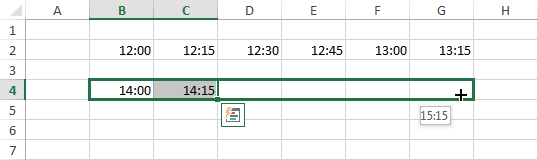
This time, you also have to select at least two values to fill the rest of the cells.

Creating Custom Lists

You might often use a list of items that are not defined in Excel. For example the list of your employees.

To create such a list in Excel, go to FILE >> Options >> Advanced >> General >> Edit Custom Lists.

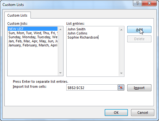
After you add your custom list, you can use it in the same way as the ones defined by Microsoft. Just type one of the values from the list, drag the mouse cursor and Excel will complete the rest.

In next tutorial i will Write about Excel 2016 Basics like Flash fill, Spell check, Undo and Redo, Hyperlinks and Data Validation. Hope that it helps for you guys.