Excel 2016 Basics Chapter 6

In this tutorials we will cover Basics of excel 2016 like Finding and replacing data, Go to special, Naming cells and ranges, and Inserting rows and columns.

Finding and replacing data in Excel 2016 Basics

When you work with Excel, sometimes you have to deal with very large amounts of data. As a result, finding a particular value can be very time-consuming. Fortunately, Excel comes with a powerful search tool, thanks to which you can quickly find the data you want.

Find

To open the Find and Replace window, go to the HOME >> Editing >> Find & Select >> Find or use one of the keyboard shortcuts: Ctrl + F or Shift + F5.

When a new window appears, you will notice that the tool in its basic form doesn’t contain many options.

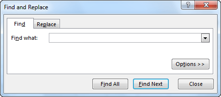
If you want to have access to more settings, click Options >> button.

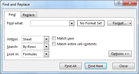
Here, you will find here three drop-down menus.

Within:

You can choose whether you want to scan for data in this sheet only or in the entire workbook.

Search:

Here, you can decide whether the values should be searched by rows or columns. This means that when a Search option is set to By Columns and you click the Find Next button, Excel will start searching in the first column and then in the next.

Look in:

You can choose whether Excel searches for data in formulas, values or comments.

Checkboxes

On the right side, you will find two checkboxes. The first one is Match case. If this option is unchecked and you start searching for the phrase “John Smith”, Excel will also return “john smith”, JOHN SMITH” or “John SMITH”. When this option is checked Excel will display the result only if the text is exactly “John Smith”.

Format

Click the Format button to set additional parameters, such as font, background, etc. For example, if you type “John Smith” and choose blue background color, then the text must meet the two conditions: it must match the phrase “John Smith” and the cell background has to be blue.

If you are not sure of the format of the cells which you are looking for, click the small triangle next to the Format button. A drop-down menu will appear. Click Choose Format From Cell… and then click on one of the cells you are interested in.

Replace

You will find a Replace button in HOME >> Editing >> Find & Select >> Replace. You can also use the Ctrl + H keyboard shortcut.

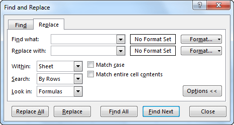
This tab is very similar to the Find tab. The difference is that in the Replace tab there is an additional textbox called Replace with. There, you can enter the text to which you want to replace the text inside the Find what text box. You can also select the formatting style.

If you don’t want to change the formatting style, but the format style is already set, you can remove it by clicking on the triangle on the Format button and then selecting Clear Replace Format.

If you want to change the formatting to normal, click on the triangle, then select Choose Format From Cell and click on the empty cell.

Go To Special in Excel 2016 Basics

Go To Special tool is used in Excel to find data of a specified type. For example formulas, text, constants, blank cells, etc.

Searching data

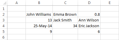
Look at the following example. This table consists of different types of data.

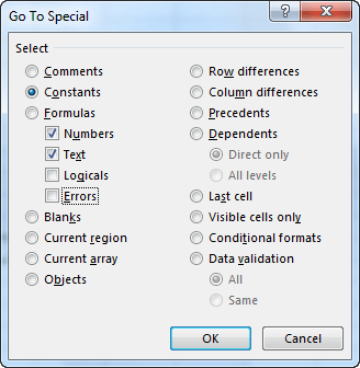
Let’s search for cells containing standard text and numbers. In order to do this, go to HOME >> Editing >> Find & Select >> Go To Special.

A new window will appear.

NOTICE

If you select a range of cells before you select Go To Special, Excel will only search those cells that are inside this range, otherwise, it will search inside the entire worksheet.

Select Constants: Numbers and Text, then confirm by clicking the OK button.

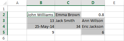
The result seems to be incorrect for two reasons:

1. Numbers inside cells B5 and D2 are not selected,
2. Date 24-May-2014 is selected.

These are not errors. Cells B5 and D2 are not constants but formulas. Cell B4 is a date, but dates in Excel are stored as numbers.

Use the Ctrl + ` keyboard shortcut to show formulas and values.

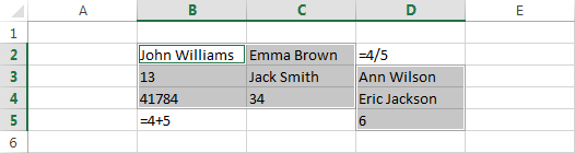
Now, you can see that Excel selected the correct cells.

Naming cells and ranges Excel 2016 Basics

When you work with worksheets, you will often type cell addresses that reference to a particular cell or a range of cells (for example, Sheet2!A3:D5). In Excel, you can name those cells to better describe their contents. For example, it is easier to understand the notation.

=SUM(cost)/month

than

=SUM(B3:B14)/D5

Naming cells

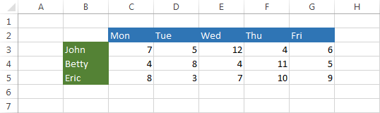
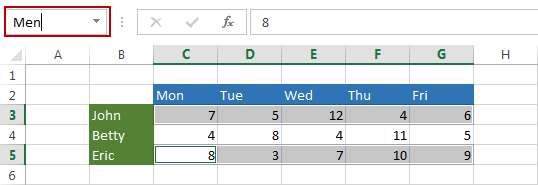
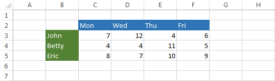
Look at the table below. There are names of three persons and the number of hours they worked each day of the week.

Let’s suppose that you want to choose all the hours worked by men at once, without selecting cells manually every time.

Example 1:

Select cells from C3 to G3, then, while holding down the Ctrl key, select cells from C5 to G5. After you do this, enter text “Men” in the Name Box.

In our example, we have only one woman. To create a named range for her, select cells from C4 to G4 and this time type “Woman” in the Name Box.

How to name multiple ranges at once

Suppose that you want to select the working hours for each day separately. You can do this in a similar way as you did it for “Men” and “Woman”. In this case, you would need to make five selections for each day separately. However, to speed up the process you can create all of them at once.

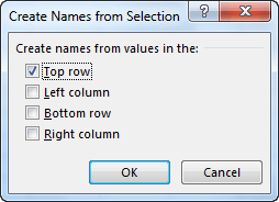
Select cells from C2 to G5, then go to FORMULAS >> Defined Names >> Create from Selection.

The Create Names from Selection window will appear, asking you which cells you want to use as names. In our case, there will be cells from the top row.

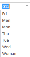
Click OK, then the arrow in the Name Box. Here, you will find two groups that you’ve created earlier: “Men” and “Woman”, as well as a group of hours for each day of the week.

Selecting ranges

There are several ways to select previously created groups.

Example 2:

The first method is to type the group name directly into a cell.

CAUTION

If you type the name =Men then Excel will return an error because you cannot enter range into one cell. In this case, you can use it in a function.

In this example, we will use the SUM function to calculate the sum of hours worked by men. When you start typing the formula, and you get to =SUM(Me, Excel will display a hint.

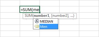
To accept this group- click it or use the Tab key.

Example 3:

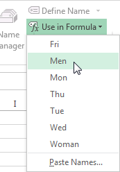
The second way is to select a group of FORMULAS >> Defined Names >> Use in formula.

Example 4:

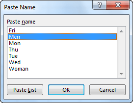
The third method is Paste Name. Press the F3 key. When a window appears, select a range from the list.

CAUTION

If you move all cells in a range, Excel will remember their new position. However, if you move only a part of them, Excel won’t be able to select them when you select a position from the Name Box.

Name manager

In the name manager, you can manage the names of ranges. You can add, delete and edit them. To use Name Manager, go to FORMULAS >> Defined Names >> Name Manager or use the Ctrl + F3 keyboard shortcut.

Insert rows and columns Excel 2016 Basics

It’s hard to plan everything in advance, so sometimes you may want to insert a new column (or row) between the existing ones.

Example 1:

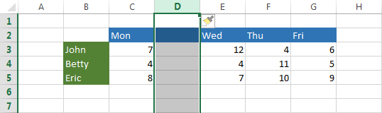
Look at the following example. There is a mistake in the table because there is “Wednesday” after “Monday”. Let’s fix it by inserting “Tuesday” between them.

In order to insert a new column, right-click the letter D and select Insert.

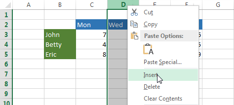
In this case, the formatting has been inherited from column C which is located to the left of the newly inserted column.

TIP

You can insert multiple columns or rows at once.

CAUTION

If there is a value in the last column (row) of the worksheet then Excel will inform you that you cannot add a new column (row) until you delete or move that value to a different location.

In next tutorial i will Write about Basics of excel 2016 like Deleting rows and columns, Hiding rows and columns, Aligning data and Cells, Adjusting text and Text orientation. Hope that it helps for you guys.